3. Propositional Logic¶

3.2.1. Validity of a Sequent¶

When multiple premises and conclusions are present they are treated as a conjunction. A sequent is said to be valid if, for every truth assignment which make the premises true, the conclusion is also true.

So for the sequent p → q , ¬ q  ⊢  ¬ p, we can construct a table like this:

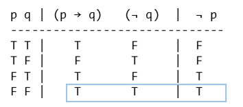
where we see that when both premises are true the conclusion is also true.

3.2.2. Logika Truth Table example¶

Logika will not support this type of proof syntax. However, with what was covered in the natural language to propositional logic lectures and the logic gates of chapter 2, we can see that this is an application of implication. We can say the sequent P1, P2, ..., Pn  ⊢ C1, C2, ... Cm is valid if the logical formula (P1 ∧ P2 ∧ ... Pn ) → (C1 ∧ C2 ∧ ... Cm ) is a tautology. Re-phrased, IF all the premises are true, THEN all consequences are true.

 1                      *
 2----------------------------
 3p q | ((p → q) ∧ ¬ q) → ¬p
 4----------------------------
 5T T |     T    F F    T F
 6T F |     F    F T    T F
 7F T |     T    F F    T T
 8F F |     T    T T    T T
 9----------------------------
10Tautology

This is discussed in more depth in the section on Soundness and Completeness, which comes later in this chapter.

Next consider the sequent ((p ∧ q) ∧ r) , s ∧ t ⊢ q ∧ t. Converted to a logic formula it is (((p ∧ q) ∧ r) ∧ (s ∧ t)) → (q ∧ t), but this will require 32 rows of truth assignments. Using inferences rules will allow us to convert this 32-line truth table proof into a 6-line proof.

3.4.1. The Two-Column Proof¶

Sequents in Logika have the following form, where premises are separated by commas.

<0 or more premises> ⊢ < 1 consequence>

Proofs are structured in 2-columns, with facts on the left and their supporting justificaiton on the right.

premises ⊢ consequent
{
    1. claim_a     justification_a
    2. claim_b     justification_b
       ...          ...
  736. consequent  justification_ef
}

Each fact is given a number, and these claim numbers are generally in order. However, the only rule is that claim numbers be unique (they may be out of order and/or non-consecutive). Also, by convention the consequence is proven on the last line, but again this is not strictly required.

Justifications are either:

3.4.2. Scope and Use of Subproofs¶

Sub-proofs are tools for case analysis or what-if excursions, used to support justification for later claims. In propositional logic, they will always contain one assumption. (In prepositional logic, their use will be expanded) This assumption is a proposition which is “local” to the sub-proof.

As a general rule, you cannot prove at the end of a sub proof the fact you assumed at the start. Assumed facts should be chosen, so that when combined with existing facts and rules, some other claim can be made at the conclusion of the sub-proof.

premises ⊢ consequent
{
   1. fact_A     justification_1
       ...          ...
   17. {
            18. fact_ D  assumption
               ...           ...
            25. fact_G   some_rule  using claim 1 // this is ok
               ...           ...
       }
       ...          ...
   45. fact_R    some_rule using claim 25   // this is not ok
}

3.7.1. Syntax¶

It is a tradition to draw the rules as a kind of “arithmetic sum-up expression”: when we have proof of the propositions above the horizontal bar, then we deduce the proposition below the bar.

The less complex rules do not include sub-proofs and have this general format.

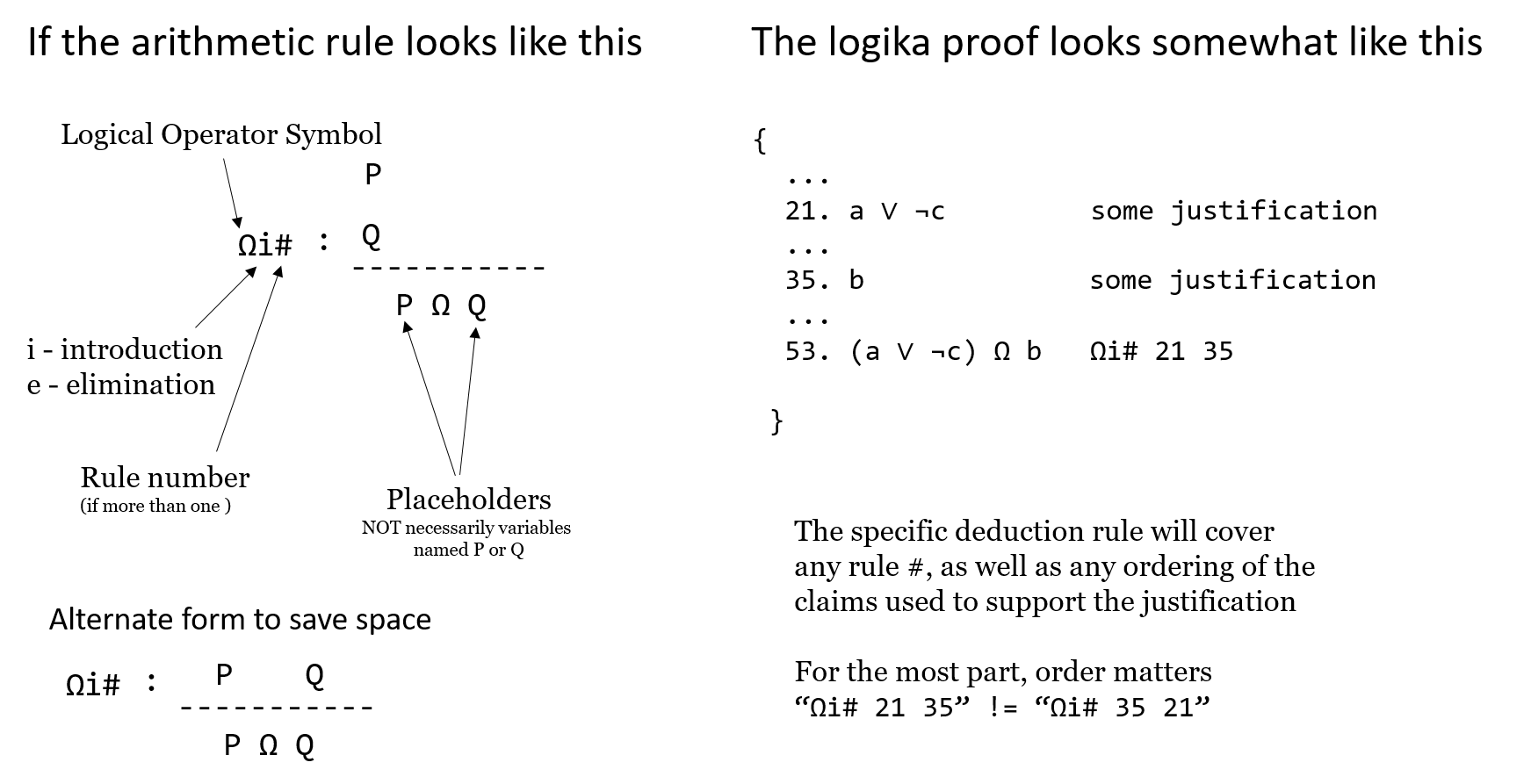
More complicated rules will involve sub-proofs and typically follow this pattern. Placeholders will be used to guide you on what must be assumed for each sub-proof.

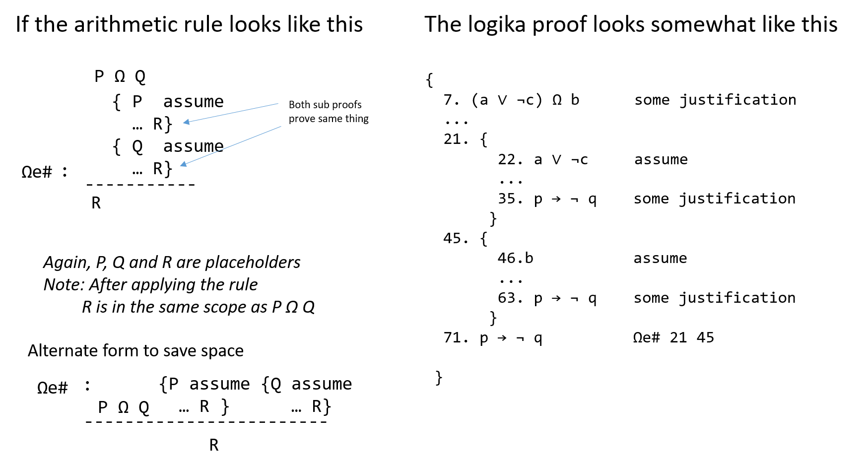
Some important things to keep in mind are:

1. Capital letters in arithmetic representations are PLACEHOLDERS not variable names.

2. Only certain rules (those with sub-proofs) let you exit a sub-proof and prove a new fact based on the sub-proof in the enclosing scope.

3.8.1. Rules¶

           P
           Q                P ∧ Q              P ∧ Q
∧i :  ---------     ∧e1 : ---------    ∧e2 : ---------
        P ∧ Q                 P                  Q

The rules are used to build proofs of new facts from starting facts (premises). The examples will explain the exact syntax.

3.8.2. Examples¶

p, q, r ⊢ r ∧ (q ∧ p)
{
  1. p                    premise
  2. q                    premise
  3. r                    premise
  4. q ∧ p                ∧i 2 1
  5. r ∧ (q ∧ p)          ∧i 3 4
}

Read line 4 like this: “from the fact stated on line 2 and the fact stated on line 1, we deduce q ∧ p by applying the ∧i law”. Lines 4 and 5 construct new facts from the starting facts (premises) on lines 1-3. A proof generates new knowledge from existing knowledge by using deduction rules.

p ∧ (q ∧ r) ⊢  r ∧ p
{
  1. p ∧ (q ∧ r)        premise
  2. p                  ∧e1 1
  3. q ∧ r              ∧e2 1
  4. r                  ∧e2 3
  5. r ∧ p              ∧i 4 2
}

The two examples seen so far suggest that a proposition like r ∧ p is like a list, (r, p), in C# that we can disassemble by indexing. The ∧e rule does the indexing, and the ∧i-does the list-building.

p ⊢ p ∧ p
{
  1. p            premise
  2. p ∧ p        ∧i 1 1
}

This example shows you can use a premise multiple times in a proof.

It is easy to prove p ∧ q ⊢ p (use ∧e1), but we cannot prove p ⊢ p ∧ q. This reminds us that deduction rules develop new knowledge, but the knowledge might be weaker than the starting facts used to deduce the knowledge. When we have propositions p and q and we prove both p ⊢ q and also q ⊢ p, we write p ⇔ q and say that p and q are equivalent – they hold the “same amounts of knowledge”.

3.8.3. Tactics¶

A tactic is a useful step towards proving a goal. The rules for conjunction come with these two tactics, which we rate from (*) to (***) based on their utility:

• (***) ∧i-tactic: If your task is to prove premises ⊢ p ∧ q, then

  1. prove Premises ⊢ p

  2. prove Premises ⊢ q

  3. use ∧i.

  The proof you are building looks like this

  1. Premises     premise
       (fill in)
  i. p
       (fill in)
  j. q
  k. p ∧  q       ∧i i j
  

• (**) ∧e-tactic: If your task is to prove Premises ⊢ r and you have as a premise or proved fact in your partial proof, p ∧ q, then apply ∧e to extract p and q to use in the proof

  1. Premises     premise
      . . .
  i.   p ∧ q      premise
  i+1. p          ∧e1 i
  i+2. q          ∧e2 i
        (fill in)
  j.   r
  

Let’s apply the tactics to one of the previous examples:

1. prove p ∧ (q ∧ r) ⊢ r∧ p: Use the (***)-∧i tactic to generate two subgoals, p ∧ (q ∧ r) ⊢ r and also p ∧ (q ∧ r) ⊢ p

   1.   p ∧ (q ∧ r)   premises
          (fill in)
   i.   r
          (fill in)
   j.   P
   j+1. r∧ p         ∧i i j
   

2. Since the (***)-tactic can’t be used on either subgoal, apply the (**)-∧e-tactic to the premise

   1.   p ∧ (q ∧ r)   premise
   2.   p             ∧e1 1     // (succeeded in proving subgoal, P)
   3.   q ∧ r         ∧e2 1
         (fill in)
   i.   r
   i+1. r∧ p          ∧i i 2
   

3. We can prove the remaining subgoal by applying the ∧e-tactic once more

   1.   p ∧ (q ∧ r)   premises
   2.   p             ∧e1 1     // (succeeded in proving subgoal, P)
   3.   q ∧ r         ∧e2 1
   4.   r             ∧e2 3     // (succeeded in proving subgoal, r)
   5.   r∧ p          ∧i 4 2
   

3.8.4. Logika Tips¶

You have to understand the order of precedence for operations. A former GTA described is as “seeing the invisible parentheses”. Consider:

p ∧ q ∧ r ⊢ r                  p ∧ q ∧ r ⊢ r
{                              {
    1. p ∧ q ∧ r premise          1. p ∧ q ∧ r premise
    2. p  ∧e1 1                   2. r  ∧e2 1
}                              }
// does not work               // works

The fact that Logika will not accept line 2 is can be irritating. One must recall that p ∧ q ∧ r is really (p ∧ q) ∧ r (from the order of precedence), and thus can be split into (p ∧ q) ∧e1 or r ∧e2.

3.9.1. Rules¶

                                                      { P assume    { Q assume
         P                  Q                 P ∨ Q     ... R    }    ... R   }
∨i1 : --------    ∨i2 :  --------        ∨e: ------------------------------------
       P ∨ Q              P ∨ Q                              R

The ∨e-rule is the deduction-rule form of case analysis: you assume p and do deductions that prove r and then you assume q and do another sequence of deductions to reprove r. Each case is a “subproof” that is indented with braces. Once both cases are proved, you conclude r no matter what. The introduction and elimination rules will be expanded on in the next section.

3.9.2. Examples¶

p ⊢ q ∨ p
{
  1. p              premise
  2. q ∨ p          ∨i2 1
}

Perhaps it seems strange to “weaken” fact p by attaching q to it. Yet, we do this all the time. For example, when we say, “today is Tuesday, so today is a weekday”, we have weakened “today is Tuesday” to “today is Monday or Tuesday or … or Friday”. In math, we might have that x > 0, so we conclude that x != 0, that is, x > 0 ⊢ (x < 0) ∨ (x > 0).

What is more interesting is that proposition q in the above proof can be any proposition, and it need not be a true fact (p is the fact that matters here). For example, we can prove 2 == 1 + 1 ⊢ (2 == 1 + 1) ∨ (1 == 0). This sequent is valid, because it is enough that 2 == 1 + 1 is a fact; literally, 1 == 0 does not matter.

A similar result goes

p ∧ q ⊢ p ∨ q
{
  1. p ∧ q        premise
  2. p            ∧e1 1
  3. p ∨ q        ∨i1 2
}

For that matter, we reprove this result using ∧e2

p ∧ q ⊢ p ∨ q
{
  1. p ∧ q        premise
  2. q            ∧e2 1
  3. p ∨ q        ∨i2 2
}

We cannot prove p ∨ q ⊢ p ∧ q, which clearly shows that the ∨i rule generates “weaker knowledge” from its facts.

Here is a proof that uses case analysis — ∨e — to prove a useful sequent.

p ∨ q, r ⊢ (p ∧ r) ∨ (q ∧ r)
{
  1. p ∨ q                     premise
  2. r                         premise
  3. {
       4. p                    assume   // (the first case for line 1)
       5. p ∧ r                ∧i 4 2
       6. (p ∧ r) ∨ (q ∧ r)    ∨i1 5
  }
  7. {
       8. q                    assume   // (the second case for line 1)
       9. q ∧ r                ∧i 8 2
       10. (p ∧ r) ∨ (q ∧ r)   ∨i2 9
  }
  11.  (p ∧ r) ∨ (q ∧ r)       ∨e 1 3 7
}

Each case — the p case and the q case — proved the same fact, so we conclude that the fact holds no matter what.

Both subproofs must prove the same fact, and then the ∨e rule finishes the proof. Here, line 11 states that, starting from the cases asserted on line 1, the proof that p proves the goal is stated in lines 4-6 and the proof that q proves the goal is stated in lines 8-10.

The assumption on line 4 (and the one on line 8) acts like a local variable inside a function – it can be used only within the function’s body. This is because the assumption is a what-if premise that is used only for the sake of discussion of the case.

Finally, here is a simple but vital proof

p ∨ p ⊢ p
{
  1. p ∨ p         premise
  2. {
       3. p        assume
  }
  4. {
       5. p        assume
  }
  6. p             ∨e 1 2 4
}

3.9.3. Tactics¶

There is one good tactic, and one not-so-good:

• (***) ∨e-tactic: To prove Premises ⊢ r, if p ∨ q appears as a premise or proved fact in the partial proof, then

  1. prove Premises, p ⊢ r

  2. prove Premises, q ⊢ r

  3. use the ∨e-rule to prove r.

  The proof is structured like this

  1. Premises       premise
       . . .
  i. p ∨ q
  j. {
       k. p         assume
            (fill in)
       l. r
  }
  m. {
       n. q         assume
            (fill in)
       o. r
  }
  p. r             ∨e i j m
  

• (*) ∨i-tactic: To prove Premises ⊢ p ∨ q, pick either of p or q, and try to prove it. Finish with ∨i

  1.  Premises     premise
       (fill in)
  i.  P
  j.  p ∨ q        ∨i1 i
  

If you examine the previous proof example, you see that the proof was constructed by applying the ∨e tactic, which made possible the use of the ∧i tactic upon the two subgoals. The ∨i tactic is used only when it is clear that it will yield progress towards the goal.

3.9.4. Logika Tips¶

Proving the exact same fact means exact. Proving p ∧ r in the first subproof and r ∧ p in the second will not work. From the Logika standpoint, these are different (at least in manual mode).

3.10.1. Rules¶

       { P assume                   P → Q
         ... Q    }                 P
→i : --------------       →e :  ------------
          P → Q                       Q

The →i-rule is a case analysis – it says, consider the case when p is a fact. (We don’t know this for certain; it is a case/possibility we want to discuss.) If assuming p (plus using other facts we already have) leads to a proof of q, then we conclude that p → q is a fact.

3.10.2. Examples¶

Here are two simple uses of →e

(p ∧ q) → r,  p → q,  p  ⊢  r
{
  1. (p ∧ q) → r           premise
  2. p                     premise
  3. p → q                 premise
  4. q                     →e 3 2
  5. p ∧ q                 ∧i 2 4
  6. r                     →e 1 5
}

(p ∨ q) → r,  q ⊢  r
{
  1. (p ∨ q) → r           premise
  2. q                     premise
  3. p ∨ q                 ∨i2 2
  4. r                     →e 1 3
}

Here is an example that uses →i

p, (q ∧ p) → r  ⊢  q → r
{
  1. p                      premise
  2. (q ∧ p) → r            premise
  3. {
       4. q                 assume
       5. q ∧ p             ∧i 4 1
       6. r                 →e 2 5
  }
  7. q → r                  →i 3
}

The proof includes the case that, when q is assumed a fact then r would follow as a fact, too. The subproof lets us conclude that q → r is a fact.

Here, two if-then facts entail a third one

p → q,  q → r  ⊢ p → r
{
  1. p → q      premise
  2. q → r      premise
  3. {
       4.  p     assume
       5.  q     →e 1 4
       6.  r     →e 2 5
  }
  7. p → r       →i 3
}

Notice how we assumed p to move the proof forwards to a proof of r. We employ a similar tactic in this example

p → (q → r) ⊢  (q ∧ p) →  r
{
  1. p → (q → r)      premise
  2. {
       3. q ∧ p       assume
       4. p           ∧e2 3
       5. q → r       →e 1 4
       6. q           ∧e1 3
       7. r           →e 5 6
  }
  8. (q ∧ p) →  r     →i 2
}

It is possible to nest cases-analyses, as in this crucial example

p → r,  q → r  ⊢  (p ∨ q) → r

{
  1. p → r             premise
  2. q → r             premise
  3. {
       4. p ∨ q        assume
       5. {
            6. p       assume
            7. r       →e 1 6
       }
       8. {
            9.  q      assume
            10. r      →e 2 9
       }
       11. r           ∨e 4 5 8
  }
  12. (p ∨ q) → r     →i 3
}

Here, the “or reasoning” is nested inside the “implies reasoning”. This example shows how mastery of basic deduction rules allows one to reason far more precisely than ordinary people do in real life.

3.10.3. Tactics¶

Implication comes with two good tactics:

• (***) →i-tactic: To prove Premises ⊢ p → q,

  1. assume p

  2. prove Premises, p ⊢ q

  3. use →i.

  The proof structure looks like this

  1.  Premises          premise
         . . .
  j.  {
        k.  p           assume
             (fill in)
        l.  q
  }
  m.  p → q            →i j
  

• (*) →e-tactic: To prove Premises ⊢ r, if p → q appears as a premise or a proved fact in the partial proof, then

  1. prove Premises ⊢ p

  2. use →e to deduce q

  3. prove Premises, P, q ⊢ r.

  Here, the tactic is to generate new knowledge that will bring us closer to the goal, r.

  1.  Premises      premise
         . . .
  i.  p → q
          (fill in)
  j.  P
  k.  q             →e i j
          (fill in)
  k.  r
  

In an earlier proof example, you see an immediate use of the (***)-→i tactic to the new subgoal

p → (q → r), q ∧ p ⊢ r

An easy application of the (**)-∧i tactic generates this simpler subgoal

p → (q → r), q, p ⊢ r

and we quickly finish the proof by applying the (*)-→e tactic twice to deduce r.

3.11.1. Rules¶

We use this symbol — ⊥ (Logika Symbol: False) — to stand for a contradiction. There is an extra rule to deduce you have proved a contradiction

        P
        ¬ P
¬ e :  -----------
         ⊥

(The name is not ideal, but we will use it anyway.)

If you start from some premises and you prove a contradiction, it means that the premises disagree with each other. (For example, from premises x > 0 and x < 0 we can deduce x > 0 ∧ ¬ (x > 0). The problem is that the premises disagree about what is true at the start.)

When we encounter a contradiction in real life, we usually “start over” and try our reasoning again, from a different set of premises. In logic, contradictions are not only a signal that we should “start over” (that is, change the premises of the proof we are building), but they are also useful for finishing a line of logical reasoning where we must consider all cases, even the impossible ones, that follow from some starting set of premises.

There is a special law for reasoning forwards from an impossible situation — the ⊥e law — which says, in the case of a contradiction, everything becomes a fact. (That is, “if False is a fact, so is everything else!”.)

         ⊥
⊥e :  ------  for any proposition, Q, at all
         Q

3.11.2. Examples¶

The ⊥e-rule works well with case analysis, where we discover that one case is impossible. Here is the classic example

p ∨ q, ¬ p ⊢ q

{
  1. p ∨ q      premise
  2. ¬ p        premise
  3. {
       4. p     assume
       5. ⊥     ¬e 4 2
       6. q     ⊥e 5
  }
  7. {
       8. q     assume
  }
  9. q          ∨e 1 3 7
}

Considering the premise, p ∨ q, we develop the two-case analysis. The first case, where p holds true, is impossible, because it causes a contradiction. The ⊥e-rule lets us gracefully prove q in this “impossible case”. (You can read lines 4-6 as saying, “in the case when p might hold true, there is a contradiction, and in such an impossible situation, we can deduce whatever we like, so we deduce q to finish this impossible case”.)

The second case, that q holds true, is the only realistic case, and it immediately yields the consequent. The proof finishes the two-case analysis with a step of ∨e.

In the ¬e rule, the positive (not negated) claim goes first.

Here is another example

p → ⊥ ⊢  p → r

{
  1. p → ⊥       premise
  2. {
       3. p      assume
       4. ⊥      →e 1 3
       5. r      ⊥e 4
  }
  6. p → r       →i 2
}

The sequent can be read as, “if p generates a contradiction, then p generates anything we want!”. Here is a more interesting variation

¬ p ⊢  p → q

{
  1. ¬ p       premise
  2. {
       3. p    assume
       4. ⊥    ¬e 3 1
       5. q    ⊥e 4
  }
  6. p → q     →i 2
}

That is, if p is impossible, we can make any old if-then claim we want about would follow if p somehow became a fact. (Example: “if I am the president of the U.S., then everyone gets a tax refund of a million bucks”. It’s a true statement but not so useful, since I am not the president and will never be.)

3.11.3. Tactic¶

• (*) ⊥-tactic: To prove Premises ⊢ q, if ¬ p appears as a premise or as a proved fact in our partial proof, then

  1. prove Premises ⊢ p

  2. use ¬ e to deduce ⊥

  3. use the ⊥e-rule to deduce q.

The structure is

1.   Premises     premise
       . . .
i.   ¬ P
      (fill in)
j.   P
k.   ⊥          ¬ e i j
l.   q            ⊥e k

In the previous proof example, we see that ¬ p ⊢ p → q is proved quickly once we obtain as a new fact (via an assumption, thanks to the (***)-→i tactic!).

3.12.1. Rule¶

       { P assume
         ... ⊥  }
¬ i:   --------------
           ¬ P

The rule says that we can discuss the case when p holds; if a contradiction results, then it is impossible for p to ever be a fact – indeed, ¬ p is the fact that holds.

3.12.2. Examples¶

p,  q → ¬ p  ⊢  ¬ q

{
  1. p           premise
  2. q → ¬ p     premise
  3. {
       4. q      assume
       5. ¬ p    →e 2 4
       6. ⊥      ¬e 1 5
  }
  7. ¬ q         ¬i 3
}

Here, the premises, p and q → ¬ p, are so strong that it is impossible for q to ever be proved as a fact. (Lines 4-5 show that, if q ever was proved a fact, it would cause a contradiction/crash.) So, ¬ q (”q is impossible”) is proved, instead.

p ⊢ ¬ ¬ p

{
  1. p           premise
  2. {
       3. ¬ p    assume
       4. ⊥      ¬e 1 3
  }
  5. ¬ (¬ p)     ¬i 2
}

Note that the ¬ i rule is not capable of proving ¬ ¬ p ⊢ p. Indeed, if “it is impossible that it is impossible for p to be a fact”, does this mean that p (is proved to be) a fact? (Example: Last night, you came home late and used your keys to enter your apartment. This morning, you can’t find your keys. You say, “It’s not that I don’t have my keys!” But do you have them in hand – do you have the evidence that you have your keys In mathematics, there are number problems where people have proved that it is impossible for there not to be a solution. But no one yet knows exactly what the solution is!)

These examples support this understanding of ¬ p

¬ p says that “p is impossible”

The three rules, ⊥e, ¬ i, and ¬ e, give the meaning of “is impossible” to the operator, ¬.

3.12.3. Tactic¶

The (***)-¬ i tactic says, to prove Premises ⊢ ¬ p,

1. assume p

2. prove Premises, p ⊢ ⊥

3. use ¬ i

1. Premises         premises
     . . .
j. {
     k.  p          assume
           (fill in)
     l.  ⊥
}
m. ¬ p                ¬ i j

The ¬ i-tactic was used with good success in the previous example.

3.13.1. Rule¶

        { ¬ P assume
          ... ⊥   }
pbc:   ---------------
             P

The pbc (“proof by contradiction”) rule says that, when ¬ p leads to a contradiction, then we have built a proof of p.

That is, when “p is impossible” is impossible, pbc concludes not only that “p is possible” but that “p is a certainty” – a fact.

In a sense, pbc builds “something from nothing” – a “proof” of “fact” p from an argument that says ¬ p leads to an impossible situation. But does this mean we have “built” p? In a world where the word “not” means the “opposite of”, we have.

3.13.2. Examples¶

¬ ¬ p ⊢ p

{
  1. ¬ ¬ p       premise
  2. {
       3. ¬ p    assume
       4. ⊥      ¬e 3 1
  }
  5. p           pbc 2
}

¬ (¬ p ∨ ¬ q)  ⊢ p ∧ q

{
  1. ¬ (¬ p ∨ ¬ q)    premise
  2. {
       3. ¬ p         assume
       4. ¬ p ∨ ¬ q   ∨i1 3
       5. ⊥           ¬e 4 1
  }
  6. p                pbc 2
  7. {
       8.  ¬ q        assume
       9.  ¬ p ∨ ¬ q  ∨i2 8
       10. ⊥          ¬e 9 1
  }
  11.  q              pbc 7
  12.  p ∧ q          ∧i 6 11
}

Here is a famous consequence of pbc: from no starting premises at all, we can prove p ∨ ¬ p for any proposition we can imagine.

⊢ p ∨ ¬ p

{
  1. {
       2. ¬ (p ∨ ¬ p)    assume
       3. {
            4. p         assume
            5. p ∨ ¬ p   ∨i1 4
            6. ⊥         ¬e 5 2
       }
       7.  ¬ p           ¬i 3
       8.  p ∨ ¬ p       ∨i2 7
       9.  ⊥             ¬e 8 2
  }
  10. p ∨ ¬ p            pbc 1
}

This is sometimes referred to as the law of the excluded middle (LEM) as p is either true or false. There is no third possibility (hence excluded middle). Now that we have done this proof, say that p stands for “God has red hair”. We have this result:

⊢ "God has red hair" ∨ ¬ ("God has red hair")

Do you accept this? Perhaps the pbc rule is not so well suited for deductions in the world of theology. A similar example is this one: let p stand for “I have stopped kicking my dog”. (But perhaps I do not even have a pet, let alone ever kicked one!)

pbc constructs “something from nothing”. This appeals to circuit builders, where ¬ and ∨ are just gates/on-off switches, but not always to computer scientists, who like to compute/build data values and data structures in constructive ways, with algorithms. For this reason, some logicians (actually, not so many) refuse to accept the pbc rule, except in specific circumstances.

Typically, when people accept that ⊢ p ∨ ¬ p is a fact, it is because they are using a decision procedure to answer the question. When we consider situations that do not have decision procedures, the situation gets murky, as in the example about the color of God’s hair.

Here is a surprising result, due to pbc

p → q ⊢ ¬ p ∨ q

 {
   1. p → q               premise

   2. {                             // start of previous p ∨ ¬ p proof
         3. ¬ (p ∨ ¬ p)   assume
         4. {
              5. p        assume
              6. p ∨ ¬ p  ∨i1 5
              7. ⊥        ¬e 6 3
         }
         8.  ¬ p          ¬i 4
         9.  p ∨ ¬ p      ∨i2 8
         10. ⊥            ¬e 9 3
   }
   11. p ∨ ¬ p            pbc 2    // conclusion of p ∨ ¬ p proof

   12. {
         13. p            assume
         14. q            →e 1 13
         15. ¬ p ∨ q      ∨i2 14
   }
   16. {
         17. ¬ p          assume
         18. ¬ p ∨ q      ∨i1 17
   }
   19. ¬ p ∨ q            ∨e 11 12 16
 }

This proof says that the dependency of q on p forces us to conclude that either q is already a fact or p is impossible. It is slightly odd that an “if-then” dependency would ensure either of the two outcomes. But this is the consequence of pbc’s ability to build something from nothing.

This result also relies on pbc

⊢ (p → q) ∨ (q → P)

for any choice whatsover of propositions p and q. (An example: let p stand for “It is raining” and q stand for “I am the President”. The above sequent holds true, even though there is no dependency between the two propositions. Why is that so? Is it reasonable? The claim looks more benign when we restrict p and q to be propositions about logic gates. The moral is, certain logic rules are meant for certain application areas, and the pbc rule works well in only circuit-theory-like worlds.)

This last result follows because pbc lets us deduce that p → q ⊢ ¬ p ∨ q – no longer does p → q tell us that p gives the needed knowledge for constructing/deducing q; no longer does p → q tell us that q physically depends on p. Instead, due to pbc, we must read p → q as stating a coincidence about the underlying True/False values of p and q. For this reason, the → operator is no longer necessary in a logic that uses the pbc rule; this is why there is no need for an → gate in circuit theory (you use ¬ p ∨ q instead).

There is no truly useful tactic for applying the pbc-rule. It is indeed a rule of “last resort”, because it says, to try to prove Premises ⊢ p, one should assume ¬ p and see if this leads one into a contradiction, that is, a proof that Premises, ¬ p ⊢ ⊥. This is a kind of logical “wild-goose chase”. But later in the chapter, we will see how computers can be made to chase after such geese.